The rescaled bootstrap

Dennis M. Feehan

2026-03-09

Introduction

This vignette demonstrates the basic functionality of the surveybootstrap package. The goal is to illustrate how to use the rescaled bootstrap (Rao and Wu 1988; Rust and Rao 1996) to take bootstrap resamples from a survey dataset when the survey sample has a complex design.

The rescaled bootstrap handles complex designs by resampling at the level of the primary sampling unit (PSU) and adjusting the sampling weights of every observation in each bootstrap replicate. Specifically, for each bootstrap resample, we draw $m_i = n_i - 1$ PSUs with replacement from the $n_i$ PSUs in stratum $i$, and rescales the observation weights to reflect how many times each PSU was selected.
This package implements the rescaled bootstrap in C++ (via Rcpp) for speed.

Use rescaled.bootstrap.sample / bootstrap.estimates when your survey has a cluster or stratified design. For a simple random sample without clusters or strata, use srs.bootstrap.sample instead.

---

The MU284 example data

The MU284 dataset (Sarndal, Swensson, and Wretman 2003, pg. 652) describes 284 Swedish municipalities. Relevant columns include:

Column	Description
LABEL	Municipality ID
S82	Total seats in municipal council
RMT85	Municipal tax revenue, 1985 (in millions of Kronor)
P85	Population, 1985 (in thousands)
CL	Cluster indicator (a set of neighboring municipalities)

MU284.complex.surveys is a list of 10 sample surveys drawn from this population using the two-stage design from Example 4.3.2 of Sarndal et al.:

• Stage I — simple random sample without replacement of $n_I = 5$ PSUs (clusters) from $N_I = 50$ total PSUs
• Stage II — simple random sample without replacement of $n_i = 3$ municipalities from each selected PSU

This gives $n = 15$ sampled municipalities per survey. Each row has a sample_weight reflecting the inverse of its selection probability.

library(surveybootstrap)

survey <- MU284.complex.surveys[[1]]
head(survey[, c("LABEL", "CL", "S82", "RMT85", "P85", "sample_weight")])
#>   LABEL CL S82 RMT85 P85 sample_weight
#> 1    96 17  41    81  13      26.66667
#> 2    99 17  49   129  20      26.66667
#> 3   101 17  61   299  49      26.66667
#> 4    16  4 101  6263 653      16.66667
#> 5    18  4  61   532  59      16.66667
#> 6    19  4  41   250  27      16.66667

---

There are two ways to use the package:

• Path 1: specifying a function to produce and estimate from data with bootstrap weights
• Path 2: getting a matrix of bootstrap weights

---

Path 1: bootstrap.estimates()

bootstrap.estimates() is the highest-level interface. You supply an estimator function and a bootstrap method; it returns bootstrap replicate estimates that you can use to compute standard errors and confidence intervals.

Step 1: define an estimator

Your estimator must accept two arguments — survey.data (the resampled dataset) and weights (a vector of rescaled sampling weights) — and return a named data frame with one row.

my_estimator <- function(survey.data, weights) {
  data.frame(
    total_S82       = sum(survey.data$S82  * weights),
    ratio_RMT85_P85 = sum(survey.data$RMT85 * weights) /
                      sum(survey.data$P85   * weights)
  )
}

Here total_S82 is the Horvitz-Thompson estimator of the population total of S82 (total council seats), and ratio_RMT85_P85 is a ratio estimator (tax revenue per capita).

Step 2: Run the bootstrap

set.seed(12345)

boot_res <- bootstrap.estimates(
  survey.data   = survey,
  survey.design = ~ CL,            # CL identifies the PSU (cluster)
  num.reps      = 500,
  estimator.fn  = my_estimator,    # we just defined this above
  weights       = "sample_weight",
  bootstrap.fn  = "rescaled.bootstrap.sample"
)

The survey.design formula uses the column CL as the PSU identifier. There are no explicit strata here, so the entire sample is treated as a single stratum. See Describing your survey design below for formulas with strata.

boot_res is a list of 500 one-row data frames, one per bootstrap replicate.

Step 3: Collect and summarize

boot_df <- do.call("rbind", boot_res)

# Bootstrap standard errors
apply(boot_df, 2, sd)
#>       total_S82 ratio_RMT85_P85 
#>    1638.2395064       0.8185707

# Bootstrap means (should be close to the original point estimates)
apply(boot_df, 2, mean)
#>       total_S82 ratio_RMT85_P85 
#>    15290.525000        8.367827

# Original point estimates for comparison
my_estimator(survey, survey$sample_weight)
#>   total_S82 ratio_RMT85_P85
#> 1     15400        8.765395

You can also pass summary.fn to bootstrap.estimates() to get a summary computed in a single pass without keeping all replicates in memory:

boot_summary <- bootstrap.estimates(
  survey.data   = survey,
  survey.design = ~ CL,
  num.reps      = 500,
  estimator.fn  = my_estimator,
  weights       = "sample_weight",
  bootstrap.fn  = "rescaled.bootstrap.sample",
  summary.fn    = MU284.estimator.summary.fn,  # example summary function
  verbose       = FALSE
)

Visualising the bootstrap distribution

hist(boot_df$total_S82,
     main  = "Bootstrap distribution: total council seats",
     xlab  = "Estimated total (S82)",
     col   = "steelblue",
     border = "white")
abline(v = my_estimator(survey, survey$sample_weight)$total_S82,
       col = "firebrick", lwd = 2, lty = 2)
legend("topright", legend = "Point estimate", col = "firebrick",
       lwd = 2, lty = 2, bty = "n")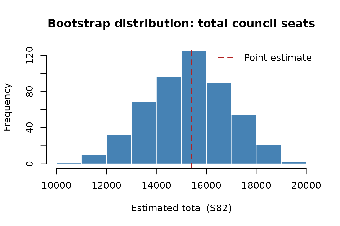

---

Path 2: get.rescaled.bootstrap.weights()

Sometimes it is more convenient to obtain a matrix of bootstrap weights directly and then apply your estimator(s) yourself. This is useful when:

• you want to compute many different estimators from the same set of replicates
• you need to pass bootstrap weights to external software
• you are implementing jackknife-after-bootstrap (JAB) variance estimation

Obtain bootstrap weights

boot_wts <- get.rescaled.bootstrap.weights(
  survey.data   = survey,
  survey.design = ~ CL,
  idvar         = "LABEL",
  weights       = "sample_weight",
  num.reps      = 500
)

The result is a list with two elements:

• orig_weights — a data frame with one row per respondent and a weight column containing the original sampling weight
• boot_weights — a data frame with one row per respondent and columns LABEL, boot_weight_1, …, boot_weight_500

names(boot_wts)
#> [1] "orig_weights" "boot_weights"

# First few rows and columns of boot_weights
boot_wts$boot_weights[1:5, 1:4]
#>   LABEL boot_weight_1 boot_weight_2 boot_weight_3
#> 1    96             0      66.66667      33.33333
#> 2    99             0      66.66667      33.33333
#> 3   101             0      66.66667      33.33333
#> 4    16             0      20.83333      20.83333
#> 5    18             0      20.83333      20.83333

Compute estimates from bootstrap weights

Join the survey data to the weight matrix, then apply your estimator for each replicate:

# Merge survey data with bootstrap weights on the respondent id
bw <- merge(survey[, c("LABEL", "S82", "RMT85", "P85")],
            boot_wts$boot_weights,
            by = "LABEL")

# Compute the total_S82 estimator for each bootstrap replicate
boot_totals <- sapply(paste0("boot_weight_", 1:500), function(col) {
  sum(bw$S82 * bw[[col]])
})

# Bootstrap standard error
sd(boot_totals)
#> [1] 1607.395

Scaling factors

Pass include_scaling_factors = TRUE to also get the per-replicate weight scaling factors. Each bootstrap weight is the product of the original weight and the corresponding scaling factor:

$$\text{boot\_weight}_{i,r} = \text{orig\_weight}_i \times \text{boot\_rep}_{i,r}$$

boot_wts_sf <- get.rescaled.bootstrap.weights(
  survey.data            = survey,
  survey.design          = ~ CL,
  idvar                  = "LABEL",
  weights                = "sample_weight",
  num.reps               = 500,
  include_scaling_factors = TRUE
)
# boot_wts_sf$weight_scaling_factor has columns LABEL, boot_rep_1, ..., boot_rep_500

---

Describing your survey design

The survey.design argument is a formula that tells surveybootstrap which columns identify PSUs and strata.

Formula	Meaning
~ CL	PSU is CL; no strata (one global stratum)
~ psu + strata(region)	PSU is psu; strata defined by region
~ psu1 + psu2 + strata(s1 + s2)	PSU uniquely identified by (psu1, psu2); strata by (s1, s2)
~ 1	Simple random sample — use srs.bootstrap.sample instead

For a simple random sample, use bootstrap.fn = "srs.bootstrap.sample" and survey.design = ~ 1:

srs_survey <- MU284.surveys[[1]]

boot_srs <- bootstrap.estimates(
  survey.data   = srs_survey,
  survey.design = ~ 1,
  num.reps      = 500,
  estimator.fn  = my_estimator,
  weights       = "sample_weight",
  bootstrap.fn  = "srs.bootstrap.sample"
)

---

Acknowledgement

DF used Claude Opus 4.6 to help improve this vignette.

References

Rao, J.N.K. and Wu, C.F.J. (1988). Resampling inference with complex survey data. Journal of the American Statistical Association, 83(401), 231–241. https://doi.org/10.1080/01621459.1988.10478591

Rao, J. N. K., C. F. J. Wu, and Kim Yue. “Some recent work on resampling methods for complex surveys.” Survey Methodology 18.2 (1992): 209-217.

Rust, K.F. and Rao, J.N.K. (1996). Variance estimation for complex surveys using replication techniques. Statistical Methods in Medical Research, 5(3), 283–310. https://doi.org/10.1177/096228029600500305

Sarndal, C.-E., Swensson, B. and Wretman, J. (2003). Model Assisted Survey Sampling. Springer. ISBN: 0387406204.